In this section I'll look at how first-order, pure integrating, and second-order processes behave when they are controlled by proportional controllers. I'll also discuss direction of control action and steady-state offset.
The algorithm for a purely proportional controller is:
![]()
or, expressed in deviation variables, the equation becomes:
![]()
the Bias term disappears in this form because it is a constant.
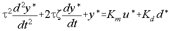
As an example, lets take a generic linear first order process expressed in deviation variables, with a single manipulation and single disturbance variable:
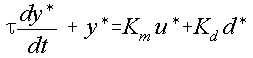
y is the controlled variable, u the manipulated variable and d the disturbance. Km and Kd are the steady-state gains on the manipulation and disturbance variables. If the controller isn't connected to the manipulation ( the process is open-loop ), the process will respond to a step change in the disturbance in a standard first-order manner. The final change in the output will be Kdd*(the change in the disturbance times the gain) and the system will take around 5*tau to reach steady-state. If, however, a proportional controller is connected to the manipulation the following results:
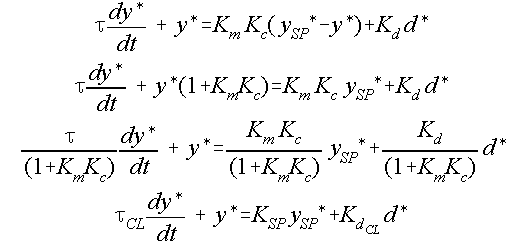
The final equation ends up as a standard form first-order differential equation - adding proportional control hasn't changed the type of response that we will obtain. What has changed is the time constant of the process which has been reduced by a factor of (1+Km Kc), the steady-state gain on the disturbance which has also been reduced by a factor of (1+Km Kc), and an extra term has been added to reflect the response to changes in the setpoint. The subscripts 'CL' mean that the terms represent the process' closed loop response - the response when the controller is connected to the process and the feedback loop is closed.
Now, let's look at what happens when the disturbance changes by a step. The process is standard first-order so we already know what the shape of the response will be. The final change in the controlled output will be :
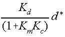
NOTE THAT PROPORTIONAL CONTROL HAS NOT ELIMINATED THE EFFECT OF THE DISTURBANCE. This is a 'feature' of proportional control which will be discussed below. What proportional control has done is to reduce the disturbance's effect by a factor of (1+Km Kc). As the controller gain becomes larger the disturbance's effect on the controlled variable becomes smaller. If an infinite gain could be used the disturbance's effect would disappear.
The other thing that has been affected in the disturbance response is the speed of response (via the time constant). The time constant has been reduced by a factor of (1+Km Kc) - as the controller gain increases, the faster the process will respond. If the gain could be made infinite the time constant would be zero and the process would eliminate disturbances instantaneously.
A movie of an example problem in proportional control is here.
The VisSim model for the example problem is here. Play with the model yourself - try to calculate the controller gain required to produce particular closed-loop gains and time constants or try to predict the effects of randomly chosen gains.
We've already seen that, with pure-first order processes, proportional control leaves a residual steady-state error on both setpoint and disturbance changes. The residual error is usually referred to as steady-state offset.
Although the maths clearly shows that steady-state offset will occur, students sometimes find it difficult to rationalise this in practical terms. A simple 'thought experiment' can help. Imagine we are trying to control the level in a tank with a manipulation on the outflow. The inflow to the tank is variable and is the process disturbance. When we start, the process is at steady-state, with zero error (the level is at the setpoint), and the controller Bias has been set so that the outflow matches the inflow. Now think of what happens if the inflow increases by a step. The only way that the process will ever come to steady-state (i.e. the level stops changing) is if the flow out of the tank precisely matches the flow into the tank. If we are using a proportional controller for level control the flow out of the tank will be determined by the equation:
![]()
Now, unless someone comes along and changes the Bias, the only way that the outflow can change to match the inflow and produce steady-state is if the error term is non-zero at steady-state. The size of this steady-state offset is affected by the controller gain - large gains will mean lower values of required offset.
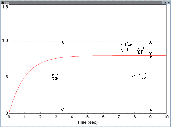
Another thing students have problems with is the difference between steady-state offsets on disturbance and setpoint changes. The steady-state offset is always the difference between the process output (controlled variable) and the setpoint when the system comes to steady-state. For disturbance changes the value of the offset is simply the closed-loop disturbance gain times the size of the disturbance change. For setpoint changes, the calculation is slightly different. For perfect setpoint tracking (error free), the steady-state gain on setpoint changes needs to be equal to one (so that, if the operator changes the setpoint by 10 degC on a temperature controller, the controlled temperature will change by 10 degC). For proportional controllers this gain will not be 1 (in most cases) and the steady-state offset can be found by taking the difference between 1 and the actual closed loop gain and multiplying this by the change in setpoint. Hopefully the graph below will make things a bit clearer!
I've already introduced the idea of control action direction from a practical viewpoint, but it can be a bit difficult to get to grips with initially when you are dealing with model equations. Ultimately, what you want to achieve is a stable closed loop equation - if you get the wrong direction of control action you'll may up making an open loop stable process closed-loop unstable! The way to avoid this is to follow this simple rule:
If the gain on the manipulated variable is positive, you need to used a reverse acting (where the error = setpoint minus measurement) controller. If the manipulation gain is negative, you need a direct acting (error = measurement minus setpoint) controller.
A pure integrating process has a model equation of the form:
Have a go at applying a proportional controller to this process, my answer is below:

There are a couple of things worth noticing here. The first is that the pure-integrating process has been converted to a first-order system. This means that the output will no longer grow without bound when the disturbance increases. The second is that the gain on setpoint changes is 1 - perfect setpoint tracking will be achieved. This is a result which will always occur under proportional control when the process contains an integrator. Note also that the disturbance has a non-zero closed-loop gain - steady-state offset will still exist when the disturbance changes.
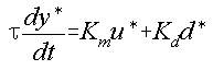
The 'standard form' of a second-order process model is:
Have a go at applying proportional control to this process yourself before revealing the solution below:

The things to notice here are:
A movie showing a worked example of proportional control of a second-order process is available here.
The model used in the move is here. Play with the model - try to calculate critical gains (the gain required to produce critical damping) for a variety of processes and see what happens in the simulation. Calculate steady-state offsets for disturbance and setpoint changes and check your answers with the simulation.